pstat
Plot statistics for a specified image section up the stack of a an IR MultiAccum image. Sections from any of the SCI, ERR, DQ, image extensions can be plotted. A choice of mean, median, mode, standard deviation, minimum and maximum statistics is available. The total number of samples is determined from the primary header keyword NSAMP and all samples (excluding the zeroth-read) are plotted. The SCI, ERR, DQ statistics are plotted as a function of sample time. The sample times are read from the SAMPTIME keyword in the SCI header for each readout.
SAMP and TIME aren’t generally populated until the FLT image stage To plot the samptime vs sample, use wfc3tools.pstat and the “time” extension
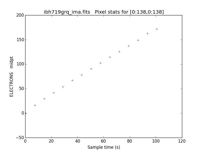
Figure 1: An example of the default plot from pstat
In [1]: pstat('ibh719grq_ima.fits')
The plotting data is returned as two arrays:
Out[2]:
(array([ 100.651947,   93.470573,   86.2892  ,   79.107826,   71.926453,
          64.745079,   57.563702,   50.382328,   43.200954,   36.019581,
          28.838205,   21.65683 ,   14.475455,    7.29408 ,    0.112705,
           0.      ]),
 array([ 171.85813415,  162.44643275,  148.99918831,  137.60458714,
         125.91510743,  114.71149769,  102.63038466,   90.97130078,
          78.26479365,   67.16825321,   53.6897243 ,   41.71639092,
          29.36628817,   16.47151355,   -0.20821257,    0.        ]))
If you want to save the plotting data into the variables time and counts you can issue the command like this:
In [1]: time,counts =pstat.pstat('ibh719grq_ima.fits')

In [2]: time
Out[3]:
array([ 100.651947,   93.470573,   86.2892  ,   79.107826,   71.926453,
         64.745079,   57.563702,   50.382328,   43.200954,   36.019581,
         28.838205,   21.65683 ,   14.475455,    7.29408 ,    0.112705,
          0.      ])

In [4]: counts
Out[5]:
array([ 171.85813415,  162.44643275,  148.99918831,  137.60458714,
        125.91510743,  114.71149769,  102.63038466,   90.97130078,
         78.26479365,   67.16825321,   53.6897243 ,   41.71639092,
         29.36628817,   16.47151355,   -0.20821257,    0.        ])
Warning
Note that the arrays are structured in SCI order, so the final exposure is the first element in the array
Parameters
- filename [file]
Input MultiAccum image name with optional image section specification. If no image section is specified, the entire image is used. This should be either a _raw or _ima file, containing all the data from multiple readouts. You must specify just the file name and image section, with no extname designation.
- extname = “sci” [string, allowed values: sci | err | dq ]
Extension name (EXTNAME keyword value) of data to plot.
- units = “counts” [string, allowed values: counts | rate]
Plot “sci” or “err” data in units of counts or countrate (“rate”). Input data can be in either unit; conversion will be performed automatically. Ignored when plotting “dq”, “samp”, or “time” data.
- stat = “midpt” [string, allowed values: mean|midpt|mode|stddev|min|max]
Type of statistic to compute.
- title = “” [string]
Title for the plot. If left blank, the name of the input image, appended with the extname and image section, is used.
- xlabel = “” [string]
Label for the X-axis of the plot. If left blank, a suitable default is generated.
- ylabel = “” [string]
Label for the Y-axis of the plot. If left blank, a suitable default based on the plot units and the extname of the data is generated.
plot = True [bool] set plot to false if you only want the data returned
Usage
pstat.py  inputFilename [pixel range]


>>> python
>>> from wfc3tools import pstat
>>> pstat(inputFilename,extname="sci",units="counts",stat="midpt",title="",xlabel="",ylabel="" )