Overview
A subset of the tools in the WFC3TOOLS package allows the user to employ the same software that STScI uses in the science calibration pipelines to calibrate WFC3 data from both the UVIS and IR detectors. This means the user can reprocess data with the latest software releases and/or reference files at will. This also means the user can customize the actual calibrations applied to the data by modifying the settings (e.g., OMIT vs PERFORM) of calibration steps in the primary header of the RAW FITS file.
The set of calibration tools resident in the WFC3TOOLS package are actually thin Python wrappers around C executables. While the C code is performing the heavy lifting, the Python wrapper acts as a convenience front-end function for the C code. In order to use the Python tools which are actually wrappers, the user must also obtain the HSTCAL package which contains the C version of the pipeline programs.
Note
While a calibration tool will be referenced generically in this discussion as, for example, calwf3, the file actually being executed in C is calwf3.e and in Python is calwf3.py/calwf3.pyc.
calwf3
The WFC3 calibration pipeline used for processing data from the UVIS or IR detectors is called calwf3. While calwf3 is a single executable which can fully process WFC3 data, the pipeline has been designed such that a number of its components can also be invoked as standalone executables. Aside from the calwf3 executable itself, the standalone executable components are: wf3cte, wf3ccd, wf32d, wf3ir, wf3rej, and wf3sum. The first three components apply to UVIS data, wf3ir applies to IR data, and the wf3rej program is used for data from both detectors to combine multiple exposures contained in a CR-SPLIT or REPEAT-OBS set. The wf3sum program sums together the IMSET chips of REPEAT-OBS exposures, and there is no Python wrapper for the wf3sum executable.
The calwf3 processes exposures according to the setting (PERFORM, OMIT, COMPLETE, SKIPPED) of the calibration switch keywords (e.g., FLATCORR, PCTECORR) in the primary header of the input file. The calibration switch keywords directly correspond to calibration processing steps. A flow diagram representing the calibration steps for the UVIS data is Fig. 3, while the complementary diagram for the IR data is Fig. 4.
The calibrated output products generated by calwf3 for UVIS are the FLT and CRJ (when applicable) files, as well as the Charge Transfer Efficiency corrected (CTE-corrected) versions of these files, FLC and CRC. Correspondingly, the output products for the IR detector are the FLT and CRJ (when applicable) files.
HST File Naming Convention available through the archive has a thorough description of how files are named and what those names mean. See also the Types of Output Files From calwf3 section in this document.
Note
For completeness of this discussion, AstroDrizzle functionality has been part of the automated calibration pipeline since 2012. AstroDrizzle removes geometric distortion, corrects for sky background variations, flags cosmic-rays, and combines images with optional subsampling. AstroDrizzle generates the calibrated drizzled data products DRZ and DRC, where the latter is for CTE-corrected images. See the WFC3 Data Handbook or DrizzlePac for more information.
As previously noted, the HSTCAL package is needed to support the calibration interface wrappers contained in the WFC3TOOLS package.
Discussion of the C Version of calwf3
Where to Find calwf3
The C code for calwf3 is part of HSTCAL package, and the source code can be downloaded from its Git repository Spacetelescope/hstcal. Downloading the source code requires compiling and linking the package with third-party software which can sometimes be tricky. Alternatively, the HSTCAL binaries can be downloaded from conda-forge. High-level release notes for all of the HSTCAL package updates can be found in its Git repository at Releases.
The current WFC3 Data Handbook can be found here. If you have questions not addressed in this documentation or need help with installing or using the software in a timely fashion, please contact the STScI Help Desk. You may also submit a GitHub issue for either the HSTCAL or WFC3TOOLS repositories.
Running calwf3
The calwf3 C executable can be run on a single input RAW file or an ASN table listing the members of an association.
When processing an association, it retrieves calibration switch and reference file keyword settings from
the first image listed in the ASN table. calwf3 does not accept a user-defined list of input images or
wildcards on the
command line (e.g. *_raw.fits cannot be used to process all raw files in the current directory).
A more extensive discussion regarding required input and options for calwf3 follows in the next
section.
The wf3ccd, wf32d, wf3cte and wf3ir tasks on the other hand, will accept
user-defined input file lists, but they will not accept an association table (_asn.fits) as input.
The standalone components wf3rej and wf3sum do not accept lists.
Command Line Options for the calwf3 C Executable
calwf3 can be called directly from the operating system command line by supplying the executable calwf3.e with an input file and a list of options. This is the same executable that the WFC3TOOLS package wraps with Python code.
   calwf3.e [options] input
   calwf3.e -vts iaa012wdq_raw.fits

   input : str
       Name of input file
       - single filename (_raw.fits or _crj.fits)
       - filename of an ASN table (_asn.fits)

   options
       -d : print optional debugging statements
       -q : print messages only to the trailer file
       -r : print version number and date of software (e.g., Current version: 3.6.2 (May-27-2021))
       -s : save temporary files
       -t : print a detailed time stamp
       -v : print verbose time stamps and information
       -1 : suppress the OpemMP parallel processing for the UVIS CTE correction
   --help : print the syntax for executing this command
--version : print version number of software (e.g., 3.6.2)
--gitinfo : print git information (if it can be obtained)
Note
calwf3 can be run on a filename which represents a single image which is not RAW (_raw.fits)
file input.
Ideally, you should use the appropriate standalone component (e.g., wf3rej) to process an
intermediate product, but calwf3 can perform this processing. This capability of calwf3
should be used with caution.
Running Many Files at the Same Time
The C command line executable only accepts one file at a time, but you can use operating system tools like
awk to process many _raw.fits files in a directory:
ls *raw.fits | awk '{print "calwf3.e",$1}' | csh
Discussion of the Python Wrapper calwf3
Where to Find calwf3
The Python wrapper for calwf3 is part of WFC3TOOLS package, and the source code can be downloaded from the Git repository in the Spacetelescope/wfc3tools area. Alternatively, the package can be downloaded from PyPi.
Running calwf3 from a Python Session Using WFC3TOOLS
The WFC3TOOLS Python wrappers act as a convenience front-end functions for the C code by allowing you to integrate the invocation of calwf3 with additional Python analysis utilities. In order to use the Python calwf3 wrapper from within the Python environment:
from wfc3tools import calwf3
filename = 'path/to/input/filename.fits'
calwf3(filename, save_tmp=True, verbose=True)
Parameter Options
input : str, default=None
Single filename (iaa012wdq_raw.fits)
Filename of an ASN table (ibfma4030_asn.fits)
- printtimebool, default=False
If True, print a detailed time stamp.
- save_tmpbool, default=False
If True, save temporary files.
- verbosebool, optional, default=False
If True, print verbose time stamps and information.
- debugbool, default=False
If True, print optional debugging statements.
- parallelbool, default=True
If True, run the code with OpemMP parallel processing turned on for the UVIS CTE correction.
- log_funcfunc(), default=print()
If not specified, the print function is used for logging to facilitate use in the Jupyter notebook.
Note
The Python calwf3 module does not support all of the command line options available to the C calwf3 executable.
Running Many Files at the Same Time
The recommended method for running calwf3 on many files is to use the calwf3 Python wrapper in the WFC3TOOLS package.
For example:
from wfc3tools import calwf3
from glob import glob

for filename in glob('i*_raw.fits'):
    calwf3(filename)
Displaying Output from calwf3 in a Jupyter Notebook
When calling calwf3 from a Jupyter notebook or from the Python wrappers, informational text output from the underlying calwf3.e C executable will be passed through print as the program runs and will show up in the user’s cell. This behavior can be customized by passing your own function as the log_func keyword argument to calwf3. As output is read from the underlying program, the calwf3 Python wrapper will call log_func with the contents of each line. The print is an obvious choice for a log function, but this also provides a way to connect calwf3 to the Python logging system by passing the logging.debug function or similar.
If log_func=None is passed, informational text output from the underlying program will be ignored, but the program’s exit code will still be checked for successful completion.
Note
When running in the notebook or from the Python wrappers, the calwf3 module may raise a RuntimeError if the underlying calwf3.e program fails with a non-zero exit code. Review the text output during the calibration call for hints as to what went wrong. Full runtime and error messages are printed to the terminal window and saved in the trailer file (.tra) for every run to help you diagnose the issue.
_asn file: name of an association table
_raw file: name of an individual, uncalibrated exposure
_crj file: name of any sub-product from an association table
_ima file: name of an intermediate step file (IR multiaccum), proceed with caution when using this option
While both CR-SPLIT and REPEAT-OBS exposures from an association get combined using calwf3, dithered observations from an association will be combined using AstroDrizzle. Images taken at a given dither position can be additionally CR-SPLIT (UVIS only) into multiple exposures.
When calwf3 is given an input file, it first discovers which of the above types of files it has been provided, and then ensures the specified input exists. calwf3 then checks to see which DETECTOR was in use for the data acqusition and calls the appropriate processing pipeline, either UVIS or IR.
Association Tables
An association file has a single extension that is a binary FITS table. The table has three columns where the member names (MEMNAME), member types (MEMTYPE), the role which that member plays in the association, and a boolean value for whether the member is present (MEMPRSNT) are displayed. The present value for the product shows “yes” because the data has already been processed and the table updated. calwf3 will check for the existence on disk of each member and then record the type and any products which will be produced from the association.
MEMTYPE |
DESCRIPTION |
|---|---|
EXP-CRJ |
An input CR-SPLIT exposure |
EXP-CRn |
An input CR-SPLIT exposure for CR-combined image n (multiple sets) |
PROD-CRJ |
CR-combined output product from a single set |
PROD-CRn |
CR-combined output product n from multiple sets |
EXP-RPT |
An input REPEAT-OBS exposure for a single set |
EXP-RPn |
An input REPEAT-OBS exposure for repeated image n |
PROD-RPT |
An output product for a REPEAT-OBS combined single set |
PROD-RPn |
REPEAT-OBS combined output product n from multiple sets |
EXP-DTH |
An input dithered exposure |
PROD-DTH |
A dither-combined output product |
In order to create a geometrically correct, drizzle-combined product, PROD-DTH exposures are combined only with AstroDrizzle, which executes after calwf3 has finished processing all members.
PROD-RPT and PROD-CRJ products are combined using wf3rej and all output files
have the _cr.fits extension.
Here’s an example of what an association table might contain:
#  Table iacr51010_asn.fits[1]  Tue 15:23:02 25-Apr-2017

# row MEMNAME        MEMTYPE        MEMPRSNT
#

    1 IACR51OHQ      EXP-RP1        yes
    2 IACR51OJQ      EXP-RP1        yes
    3 IACR51OKQ      EXP-RP2        yes
    4 IACR51OMQ      EXP-RP2        yes
    5 IACR51010      PROD-DTH       yes
    6 IACR51011      PROD-RP1       yes
    7 IACR51012      PROD-RP2       yes
The association file has four REPEAT-OBS exposures and instructs calwf3 to make three products, one for RP1 members, one for RP2 members, and one dither combination for all of the members.
The IACR51010 will be produced by AstroDrizzle while the IACR51011 and IACR51012 products will be produced by calwf3 using wf3rej.
Intermediate Files
When calwf3 determines that an intermediate product has been given as input, the preferred method is for users to call the stand-alone tasks by hand. However, it will default to looking for the ASN_TAB keyword in the file header and will partially process the table that is specified.
Single Files
As previously noted, the calwf3 processes exposures according to the calibration switch settings in the primary header of the input file. For single exposure processing, the calibration switch keywords, CRCORR and RPTCORR, are set to OMIT by default, as these processes require multiple observations.
UVIS Data Single File FITS Format
The full-frame _raw.fits file for the UVIS detector data contains a primary
header data unit (PHDU) with global header information and no data component,
as well as multiple extensions in groups of three. Each exposure has a corresponding
set of three extensions that are comprised of
the science image itself, the error associated with each pixel, and data quality flags
for the pixel.
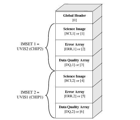
Fig. 1 UVIS data raw file format
IR Data Single File FITS Format
The input _raw.fits file for the IR detector data also contains a primary
header data unit (PHDU) with global header information and no data component,
as well as multiple extensions in groups of five. In this case each exposure has
a corresponding set of five extensions that are comprised of the science image itself,
the error associated with each pixel, data quality flags for the pixel, the number of
samples used to calculate the pixel signal, and the accumulated integration time for
each pixel. The final output file contains only five extensions, each containing the
final values for the entire set of exposures as related to the slope image in the science
extension.
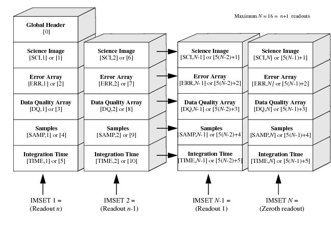
Fig. 2 IR data raw file format
Explanation of the FITS Extensions
The science image contains the data from the focal plane array detectors.
The error array contains an estimate of the statistical uncertainty associated with each corresponding science image pixel
The data quality array contains independent flags indicating various status and problem conditions associated with each corresponding pixel in the science image
The sample array (IR ONLY) contains the number of samples used to derive the corresponding pixel values in the science image.
The time array (IR ONLY) contains the effective integration time associated with each corresponding science image pixel value.
Types of Output Files from calwf3
The suffixes used for WFC3 raw and calibrated data products closely align to those used by ACS and NICMOS:
SUFFIX |
DESCRIPTION |
UNITS |
|---|---|---|
_raw |
raw data |
DN |
_rac |
UVIS CTE corrected raw data, no other calibration |
DN |
_asn |
association table for observation set |
|
_spt |
telescope and WFC3 telemetry and engineering data |
|
_blv_tmp |
overscan-trimmed UVIS exposure |
DN |
_blc_tmp |
overscan-trimmed UVIS, CTE corrected exposure |
DN |
_crj_tmp |
uncalibrated, cosmic-ray rejected combined |
DN |
_crc_tmp |
uncalibrated, cosmic-rat rejected, CTE cleaned |
DN |
_ima |
calibrated intermediate IR multiaccum image |
\(e^{-}/s\) |
_flt |
UVIS calibrated exposure |
\(e^{-}\) |
_flc |
UVIS calibrated exposure including CTE correction |
\(e^{-}\) |
_flt |
IR calibrated exposure |
\(e^{-}/s\) |
_crj |
UVIS calibrated, cosmic ray rejected image |
\(e^{-}\) |
_crj |
IR calibrated, cosmic ray rejected image |
\(e^{-}/s\) |
_crc |
UVIS calibrated, CR rejected, CTE cleaned image |
\(e^{-}\) |
.tra |
trailer file, contains processing messages |
The DRZ and DRC products are produced with AstroDrizzle which executes once calwf3 completes.
Keyword Usage
calwf3 processing is controlled by the values of keywords in the input image headers. Certain
keywords, referred to as calibration switches, are used to control which calibration steps are
performed. Reference file keywords indicate which reference files to use in the corresponding
calibration steps. Users who wish to perform custom reprocessing of their data may change
the values of these keywords in the _raw.fits file primary headers and then rerun the
modified file through calwf3. See the
WFC3 Data Handbook
for a more complete description of these keywords and their values.
Using CRDS to Update Your Reference Files
CRDS is the reference file management software used by STScI for organizing and assigning reference files to datasets. Users can query CRDS to get the best reference files for their data available at the time of the request. The following link explains how you can use this facility via a web interface, Using CRDS to find the best reference files for your data, or from the command line.
UVIS Pipeline
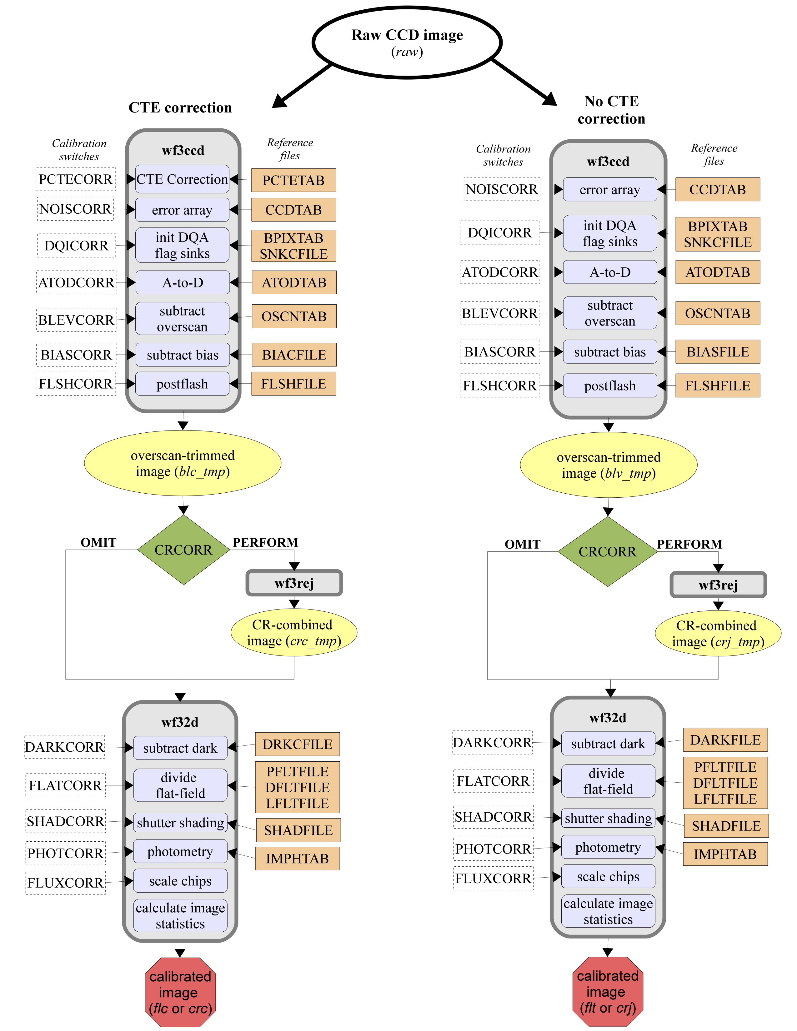
Fig. 3 Flow diagram for calwf3 data. wf3cte occurs as the very first step, before wf3ccd.
As of calwf3 v3.3, the calwf3 pipeline processes all UVIS data twice, once with the CTE correction applied as the first step, and a second time without the CTE correction. A short description of the calibration steps, in the order they are performed:
Calculate and remove and CTE found in the image (PCTECORR)
Calculate a noise model for each pixel and record in the error array (ERR) of the image (NOISCORR)
Initialize the data quality (DQ) array of the image based on BPIXTAB , flag A-to-D saturation, and potentially flag full-well saturation (DQICORR)
Correct for A-to-D conversion errors where necessary, currently skipped (ATODCORR)
Subtract bias level determined from overscan regions (BLEVCORR)
Subtract the bias image (BIASCORR)
If applicable, employ a full-well saturation image, SATUFILE, to flag affected pixels.
Detect and record SINK pixels in the DQ mask (performed if DQICORR is set to PERFORM)
Subtract the post-flash image, if applicable (FLSHCORR)
Scale and subtract the dark image (DARKCORR)
Perform flatfielding and unit conversion (FLATCORR)
Perform shutter-shading correction where necessary, currently skipped (SHADCORR)
Populate photometric header keywords (PHOTCORR)
Calculate image statistics for the header
Correct chips to be on the same zeropoint (FLUXCORR)
Calculate basic pixel statistics for the image and store the values in relevant header keywords (no switch)
The ATODCORR step is currently skipped as WFC3 ground tests did not show a bias toward the assignment of certain DN values, so this correction is not needed. The SHADCOR step which corrects the science image for differential exposure time across the detector caused by the amount of time it takes for the shutter to open and close completely is an insignificant effect. This step is always set to OMIT.
If BLEVCORR and BIASCORR are performed, a full-well saturation image (SATUFILE) is applied to flag affected pixels. This is the updated and preferred method of flagging such pixels. If the SATUFILE keyword is missing from the FITS header, then the flagging of full-well saturated pixels is done during the DQICORR step using a single constant value as the threshold.
Correction For Charge Transfer Efficiency (PCTECORR)
The charge transfer (CTE) of the UVIS detector has been declining over time as on-orbit radiation damage creates charge traps in the CCDs. Faint sources, in particular, can suffer large flux losses or even be lost entirely if observations are not planned and analyzed carefully. The CTE depends on the morphology of the source, the distribution of electrons in the field of view, and the population of charge traps in the detector column between the source and the transfer register. Further details regarding the understanding of the WFC3/UVIS charge transfer efficiency (CTE) are presented in several documents. Please see WFC3 ISR 2021-13, as well as other ISRs found in the WFC3 documentation <https://www.stsci.edu/hst/instrumentation/wfc3/documentation/instrument-science-reports-isrs>`_. The PCTECORR step aims to mitigate the flux loss incurred from CTE.
More information on this part of the pipeline can be found in the wf3cte documentation.
Error Array Initialization (NOISCORR)
The image error array is initialized. The function examines the ERR extension of the input data to determine the state of the array. The input _raw image contains an empty ERR array. If the ERR array has already been expanded and contains values other than zero, then this function does nothing. Otherwise it will initialize the ERR array by assigning pixel values based on a simple noise model. The noise model uses the science (SCI) array and for each pixel calculates the error value \(\sigma\) in units of DN: The NOISCORR calibration step keyword is not explicitly listed in the image header (i.e., it is not user-accessible), and it is always set to PERFORM.
The CCDTAB reference file contains the bias, gain and readnoise values used for each CCD amplifier quadrant used in this calculation. The table contains one row for each configuration that can be used during readout, which is uniquely identified by the list of amplifiers (replicated in the CCDAMP header keyword), the particular chip being read out (CCDCHIP), the commanded gain (CCDGAIN), the commanded bias offset level (CCDOFST) and the pixel bin size (BINAXIS). These commanded values are used to find the table row that matches the characteristics of the image that is being processed and reads each amplifiers characteristics, including readnoise (READNSE), A-to-D gain (ATODGN) and the mean bias level (CCDBIAS).
Data Quality Array Initialization (DQICORR)
This step initializes the data quality array by reading a table of known bad pixels for the detector, as stored in the Bad Pixel reference table BPIXTAB. In addition to the bad pixel types in the table, the types of bad pixels that can be flagged are:
NAME |
VALUE |
DESCRIPTION |
|---|---|---|
GOODPIXEL |
0 |
OK |
SOFTERR |
1 |
Reed-Solomon decoding error |
DATALOST |
2 |
data replaced by fill value |
DETECTORPROB |
4 |
bad detector pixel or beyond aperture |
DATAMASKED |
8 |
masked by occulting bar |
HOTPIX |
16 |
hot pixel |
CTETAIL |
32 |
UVIS CTE tail (pre-November 2012) |
CTETAIL |
32 |
UVIS unstable pixel (post-November 2012) |
WARMPIX |
64 |
warm pixel |
BADBIAS |
128 |
bad bias value |
SATPIXEL |
256 |
full-well or a-to-d saturated pixel |
BADFLAT |
512 |
bad flatfield value |
TRAP |
1024 |
UVIS charge trap, SINK pixel |
ATODSAT |
2048 |
a-to-d saturated pixel |
TBD |
4096 |
reserved for Multidrizzle CR rej |
DATAREJECT |
8192 |
rejected during image combination UVIS, IR CR rejection |
CROSSTALK |
16384 |
ghost or crosstalk |
RESERVED2 |
32768 |
cannot use |
If the newer (mid-2023) SATUFILE FITS keyword is missing or invalid in the input image header, the full-well saturated pixels are flagged during the DQICORR step using a single value as the threshold. However, the newer technique is to flag the full-well saturated pixels in a sub-step after BLEVCORR/BIASCORR using a full two-dimensional image as the threshold.
Overscan Bias Correction (BLEVCORR)
The location of the overscan regions in a raw image varies, depending upon the type of readout that is performed. The overscan regions are used to monitor the instrument as well as provide a measure of the bias level at the time the detector was exposed. The bias level which is calculated for subtraction is done on a line-by-line basis in the image. If the image has no overscan region the BIAS level to be subtracted is obtained from the CCDTAB reference file. Otherwise, the columns to use for the calculation are referenced in the OSCNTAB reference file. The OSCNTAB refers to all regions in pixel coordinates, even when the image is binned. A bias drift calculation is made if there are virtual overscan pixels which exist, if neither of the virtual overscan regions are specified, then the physical overscan region is used.
If there are two sections available to use for the line because only one amp was used, then they are averaged. The parallel overscan region is split into two if there is more than one amp. If the virtual overscan is used, a straight line is fit as a function of the column number. The fit is evaluated for each line and then subtracted from the data. Iterative sigma clipping is used to reject outliers from the array of bias values.
The mean value of all the bias levels which were subtracted is recorded in the SCI extension output header in MEANBLEV.
parallel readout direction, amp A
|
|
v
(VX1,VY1)     (VX2,VY2)
A       /         \     B
-----/-----------+---
|   |/     |      |   | } TRIMY2
|   +------+------    |
|   |      |      |   | <--- serial readout direction, amp A
|   |      |      |   |
| - | -----+------|---|<-- AMPY
|   |      |      |   |
|   |      |      |   |
|   |      |      |   |
|    ------+------    |
|   |      |      |   | } TRIMY1
---------------------
C /  \      ^       / \ D
A1  A2     |      B1  B2
  AMPX

A,B,C,D   - Amps
AMPX      - First column affected by second AMP
AMPY      - First line affected by second set of AMPS
(VX1,VY1) - image coordinates of virtual overscan region origin
(VX2,VY2) - image coordinates of top corner of virtual overscan region
A1,A2     - beginning and ending columns for leading bias section
    (BIASSECTA1,BIASSECTA2 from OSCNTAB)
B1,B2     - beginning and ending columns for trailing bias section
    (BIASSECTB1,BIASSECTB2 from OSCNTAB)
TRIMX1    - Number of columns to trim off beginning of each line,
    contains A1,A2
TRIMX2    - Number of columns to trim off end of each line,
    contains B1,B2
TRIMY1    - Number of lines to trim off beginning of each column
TRIMY2    - Number of line to trim off end of each column
Bias Correction (BIASCORR)
This step subtracts the two dimensional bias structure from the image using the superbias reference image listed in the header keyword BIASFILE. The dimensions of the image are used to distinguish between full-frame and subarray images. Because the bias image is already overscan-subtracted, it will have a mean pixel value of less than one. The BIASFILE has the same dimensions as a full-size science image, complete with overscan regions. Only after completion of wf3ccd are the science images trimmed to their final calibrated size. Since the same reference image is used for full-frame and subarray images, calwf3 will extract the matching region from the full-size bias file and apply it to the subarray image.
If both the BLEVCORR and BIASCORR steps are performed, and the input image contains a valid FITS SATUFILE keyword in the primary header, then the full-well saturation image identified by the SATUFILE keyword will be usedto define the saturation threshold for flagging at this stage.
Sink Pixel Detection and Marking
Sink pixels are a type of image defect. These pixels contain a number of charge traps and under-report the number of electrons that were generated in them during an exposure. These pixels can have an impact on nearby upstream or downstream pixels. Though they often only impact one or two pixels when the background is high, they can impact up to 10 pixels if the background is low.
Flagging of SINK pixels in the DQ extension of calibrated images is controlled with the DQICORR header keyword, happens after the bias correction has been performed, and is done in the amp-rotated C-D-A-B full image format used and described in the CTE correction. When set to perform, the sink pixels are located and flagged with help from the SNKCFILE reference image. Given the reference image, the procedure for flagging the sink pixel in science data involves:
Extract the MJD of the science exposure
Go through the reference image pixel by pixel looking for those pixels with values greater than 999, which indicates that the current pixel is a sink pixel. The value of this pixel in the reference file corresponds to the date at which this pixel exhibited the sink behavior.
If the turn on date of the sink pixel is after the exposure date of the science image, then we ignore the sink pixel in this exposure and move on to the next pixel
If the turn on date of the sink pixel is before the exposure date of the science image, then this science pixel was compromised at the time of the exposure. The corresponding DQ extension pixel for this science pixel is flagged with the “charge trap” flag of 1024.
If the pixel “below” the sink pixel in the long format image has a value of -1 in the reference image, then it is also flagged with the “charge trap” value in the DQ extension. We then proceed vertically “up” from the sink pixel and compare each pixel in the reference file to the value of the sink pixel in the science exposure at hand. If the value of the sink pixel in the exposure is below the value of the upstream pixel in the reference image, we flag that pixel with the “charge trap” value in the DQ extension. We continue to flag pixels until the value of the pixel in the reference image is zero or until the value of the sink pixel in the exposure is greater than the value of the upstream pixel in the reference image.
WFC3 ISR 2014-19 has a detailed analysis on detection of the sink pixels, while the strategy for flagging them is discussed in WFC3 ISR 2014-22.
Sink pixels were originally only flagged in full frame science images, but since calwf3 v3.4 sink pixel flagging has also been done in subarray images. The pipeline currently does no further analysis or correction on pixels which have been flagged as affected by sink pixels.
Post-Flash Correction (UVIS ONLY) (FLSHCORR)
WFC3 has post-flash capability to provide a means of mitigating the effects of Charge Transfer Efficiency (CTE) degradation. When FLSHCORR=PERFORM, this routine subtracts the post-flash reference image, FLSHFILE, from the science image step. The success of the post-flash operation during the exposure is first verified by checking the keyword FLASHSTA. The FLSHFILE is renormalized to the appropriate post-flash current level (LOW, MED, HIGH) recorded in the FLASHCUR keyword, and the flash duration (FLASHDUR) is then subtracted from the science image. The mean value of the scaled post-flash image is written to MEANFLSH in the output SCI extension header. Different members of an association can have different values of SHUTRPOS because it varies by exposure, and this is fine for calibration because the references files are populated separately for each exposure.
KEYWORD |
DESCRIPTION |
|---|---|
FLSHDUR |
is the length of time of the flash exposure |
FLSHCUR |
is the current that was used to the lamp as calculated by TRANS, which also calculates FLASHEXP, (ZERO, LOW, MED, HIGH) |
FLSHFILE |
is the flash reference file, which has an illumination pattern for each shutter |
SHUTRPOS |
says which shutter was used |
FLASHSTA |
indicates an interrupted exposure (ABORTED, SUCCESSFUL, NOT PERFORMED) |
FLASHLVL |
post-flash level in electrons |
MEANFLSH |
the mean level which calwf3 calculated and then subtracted |
- Further reading:
WFC3 Instrument Handbook Chapter 6.9.2: CTE-Loss Mitigation Before Data Acquisition
Dark Current Subtraction (DARKCORR)
The reference file listed under the DARKFILE header keyword is used as the reference dark image. In the UVIS, the dark image is scaled by EXPTIME and FLASHDUR. The reference file pointed to with DARKFILE is used for the non-CTE corrected data, while the reference file pointed to with DRKCFILE is used for the CTE corrected data.
FLATCORR
Correct the image for pixel quantum efficiency using the reference image specified by the FLATFILE keyword in the header.
This actually consists of correction using up to 3 reference flat images:
PFLTCORR: apply a pixel-to-pixel flat (ground flats)
DFLTCORR: apply a delta flat, applies any needed changes to the small-scale PFLTFILE
LFLTCORR: apply a low order flat, correcting for large scale sensitivity variations (on-orbit)
The pipeline is currently only using the P-flats. If two or more reference files are specified, they are read in line-by-line and multiplied together to form a combined flatfield correction image.
Subarray science images use the same reference file as the full-frame images; calwf3 will extract the appropriate region from the reference file and apply it to the subarray input image.
Unit Conversion to Electrons
The calibration reference flat image is divided by the calibrated gain value, and then the science image is divided by the flat.
Any calibration reference file data which is in units of electrons and is used in calwf3 prior to the unit conversion step, has the gain applied before use to ensure the calibration data and the input data are in consistent units.
Shutter Shading Correction (SHADCORR)
This step corrects the science image for differential exposure time across the detector cased by the amount of time it takes for the shutter to completely open and close, which is a potentially significant effect only for images with very short exposure times (less than ~5 seconds). Pixels are corrected based on the exposure time using the relation:
WFC3 tests have shown that the shutter shading effect is insignificant (< 1%), even for the shortest allowed UVIS exposure time of 0.5 seconds (WFC3 ISR 2007-17). Therefore this step is ALWAYS set to OMIT in calwf3.
Photometry Keywords (PHOTCORR)
The PHOTCORR step is performed using tables of precomputed values. Instead of calls to SYNPHOT, it uses the reference table specified in the IMPHTTAB header keyword. Each DETECTOR uses a different table.
If you do not wish to use this feature, set the header keyword PHOTCORR to OMIT. However, if you intend to use the FLUXCORR step, then PHOTCORR must be set to PERFORM as well.
PHOTFNU: the inverse sensitivity in units of \(Jansky\ sec\ electron^{-1}\)
PHOTFLAM: the inverse sensitivity in units of \(ergs\ cm^{-2} A^{-1} electron^{-1}\)
PHOTPLAM: the bandpass pivot wavelength \(A\)
PHOTBW: the bandpass RMS width \(A\)
PHTFLAM1: the inverse sensitivity in units of \(ergs\ cm^{-2} A^{-1} electron^{-1}\)
PHTFLAM2: the inverse sensitivity in units of \(ergs\ cm^{-2} A^{-1} electron^{-1}\)
For versions 3.3 and beyond, the value PHOTFNU is calculated specific to each UVIS chip, see the section on FLUXCORR for more information.
The SCI headers for each chip contain the PHOTFNU keyword, which is valid for its respective chip, where PHOTFNU is calculated as:
For UVIS1: \(photfnu = 3.33564 x 10^{4} * PHTFLAM1 * PHOTPLAM^{2}\)
For UVIS2: \(photfnu = 3.33564 x 10^{4} * PHTFLAM2 * PHOTPLAM^{2}\)
The IMPHTTAB file format for WFC3/UVIS is as follows:
EXT#  FITSNAME      FILENAME              EXTVE DIMENS       BITPI OBJECT

0     z7n21066i_imp z7n21066i_imp.fits                       16
1       BINTABLE    PHOTFLAM              1     5Fx256R
2       BINTABLE    PHOTPLAM              1     5Fx256R
3       BINTABLE    PHOTBW                1     5Fx256R
4       BINTABLE    PHTFLAM1              1     5Fx256R
5       BINTABLE    PHTFLAM2              1     5Fx256R
where each extension contains the photometry keyword information for that specific header keyword. The rows inside the tables are split on observation mode.
Flux normalization for UVIS1 and UVIS2 (FLUXCORR)
The FLUXCORR step was added in calwf3 v3.2 as a way to scale the UVIS chips so that the flux correction over both chips is uniform. This required new keywords which specify new PHOTFLAM values to use for each chip as well as a keyword to specify the scaling factor for the chips. New flatfields must be used and will replace the old flatfields in CRDS but the change will not be noticeable to users. Users should be aware that flatfield images used in conjunction with calwf3 v3.2 of the software should not be used with older versions as the data, and vice versa as the scaling will be incorrect.
The new keywords include:
PHTFLAM1: The FLAM for UVIS1
PHTFLAM2: The FLAM for UVIS2
PHTRATIO: The ratio: PHTFLAM2 / PHTFLAM1, which is calculated by calwf3 and is multiplied with UVIS2 (SCI,1 in the data file)
Note
In order for FLUXCORR to work properly the value of PHOTCORR must also be set to PERFORM since this populates the header of the data with the keywords FLUXCORR requires to compute the PHTRATIO.
This step is performed by default in the pipeline and the PHOTFLAM keyword will be valid for both chips after the correction has been applied.
Cosmic-ray rejection
Associations with more than one member, which have been associated using either CR-SPLIT or REPEAT-OBS, will be combined using wf3rej. The task uses the same statistical detection algorithm developed for ACS (acsrej), STIS (ocrrj) and WFPC2(crrej), providing a well-tested and robust procedure. The DRZ and DRC products will be created from the association, with AstroDrizzle, which will also correct for geometric distortion.
IR Pipeline
IR pipeline output files using the RAW file as input:
flt.fits: output calibrated, ramp-fitted exposure produced after CRCORR has been run
ima.fits: output ramp calibrated exposure. Remember that the signal rate recorded in each SCI extension of the ima file represents the average flux between that particular readout and the zero read.
_crj.fits: a cosmic-ray rejected sub-product produced from images in an association table
.tra: output text information about the processing
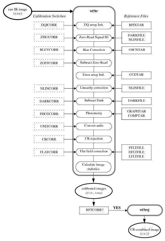
Fig. 4 Flow diagram for IR data using wf3ir in calwf3
Data Quality Initialization (DQICORR)
Initialize the data quality array for the image using the reference file specified in its header with BPIXTAB. The DQ array is no longer updated to reflect any TDF transition during the sample. If you want to update DQ pixel values yourself before running further processing, do it after this first step has been completed, remembering that the data in this extension is always in units of UNSIGNED INTEGER. The following table lists the DQ flag values and their meanings:
NAME |
VALUE |
DESCRIPTION |
|---|---|---|
GOODPIXEL |
0 |
OK |
SOFTERR |
1 |
Reed-Solomon decoding error |
DATALOST |
2 |
data replaced by fill value |
DETECTORPROB |
4 |
bad detector pixel or beyond aperture |
DATAMASKED |
8 |
masked by occulting bar |
BADZERO |
8 |
deviant IR zero-read pixel |
HOTPIX |
16 |
hot pixel |
UNSTABLE |
32 |
IR unstable pixel |
WARMPIX |
64 |
warm pixel |
BADBIAS |
128 |
bad bias value |
SATPIXEL |
256 |
full-well or a-to-d saturated pixel |
BADFLAT |
512 |
bad flatfield value |
SPIKE |
1024 |
CR spike detected during cridcalc IR |
ZEROSIG |
2048 |
IR zero-read signal correction |
ne TBD |
4096 |
reserved for Multidrizzle CR rej |
DATAREJECT |
8192 |
rejected during image combination UVIS, IR CR rejection |
HIGH_CURVATURE |
16384 |
pixel has more than max CR’s |
RESERVED2 |
32768 |
can’t use |
Estimate the signal in the zero read (ZSIGCORR)
This step measures the signal between the super zero read in the linearity reference file (NLINFILE) and the science zero read exposure, the steps are roughly as follows:
copy the zero sig image from the linearity reference file
compute any subarray offsets
subtract the super zero read reference image from the zero read science image
compute the noise in the zero image
pixels which contain more than ZTHRESH*noise of detected signal are flagged and that signal is passed to the NLINCORR step to help judge saturation and linearity, avoiding reference pixels.
low signal pixels are masked out by setting them to zero
the NLINCOR file has an extension with saturation values for each pixel which is referenced here. Pixels which are saturated in the zeroth or first reads are flagged in the DQ and the number of found saturated pixels are reported.
This step works poorly for bright targets which are already begining to saturate in the zeroth and first reads
This step acutally subtracts the super zero read from the science zero read instead of calculating an estimated signal based on the first read and zero read + estimated exposure time between them so that the difference in readout time for subarrays is not an issue.
Bias Correction (BLEVCORR)
This step subtracts the bias level using the reference pixels around the perimeter of the detector, the boundries of the reference pixels are defined in the OSCNTAB reference file. There are 5 reference pixels on each end of each row, but 1 is ignored on each side, for a total of 8 being used per row. The resistent mean of the standard deviation of all the reference pixels in the image is subtracted from the entire image and the value is stored in the MEANBLEV keyword in the output image header. The reference pixels are left in place in the IMA output image through processing, but the final FLT image has been trimmed to just the science pixels.
Zero read subtraction (ZOFFCORR)
The original zero read is subtracted from all groups in the science image, including the zeroth read itself, combining the DQ arrays with a logical OR. The ERR and SAMP arrays are unchanged and the TIME arrays are subtracted from each other. The exposure time for the group being corrected is reduced by an amount equal to the exposure time of the zero-read. At this point we’ve subtracted the mean bias using the reference pixels (BLEVCORR) and added back in the signal from the super zero read (done at the end of ZSIGCORR). What’s left in the zero read of the science image is the superbias subtracted signal. The TIME and SAMP arrays are saved to the FLT image only AFTER the CRCORR step has been completed.
Error array initialization
The errors associated with the raw data are estimated according to the noise model for the detector which currently includes a simple combination of detector readnoise and Poisson noise from the pixel. Readnoise and gain are read from the CCDTAB reference file. The ERR array continues to be summed in quadrature as the SCI array is processed. Inside the final FLT image, the ERR array is calculated by CRCORR as the calculated uncertainty of the count-rate fit to the multiaccum samples.
Detector Non-linearity Correction (NLINCORR)
The integrated counts in the science images are corrected for the non-linear response of the detectors, flagging pixels which extend into saturation (as defined in the saturation extension of the NLINFILE reference image). The observed response of the detector can be represented by two regimes:
At low and intermediate signal levels the detector response deviates from the incident flux in a way that is correctable using the following expression
where c1, c2, c3, and c4 are the correction coefficients, F is the uncorrected flux in DN and \(F_{c}\) is the corrected flux. The current form of the correction uses a third-order polynomial, but the algoritm can handle an arbitrary number of coefficients. The number of coefficients and error terms are given by the values of the NCOEFF and NERR keywords in the header of the NLINFILE.
At high signal levels, as saturation sets in, the response becomes highly non-linear and is not correctable to a scientifically useful degree.
The signal in the zero read is temporarily added back to the zeroth read image of the science data before the linearity correction is applied and before the saturation is judged. Once the correction has been applied the signal is once again removed. This only occurs if the ZSIGCORR step is set to PERFORM. Saturation values for each pixel are stored in the NODE extension of the NLINFILE. After each group is corrected, the routine also sets saturation flags in the next group for those pixels that are flagged as saturated in the current group. This is necessary because the SCI image value of saturated pixels will sometimes start to go back down in the subsequent reads after saturation occurs, which means they could go unflagged by normal checking techniques. The SAMP and TIME arrays are not modified during this step.
The format of the linearity reference file:
EXT#  FITSNAME      FILENAME              EXTVE DIMENS       BITPI OBJECT

0     u1k1727mi_lin u1k1727mi_lin.fits                       -32
1       IMAGE       COEF                  1     1024x1024    -32
2       IMAGE       COEF                  2     1024x1024    -32
3       IMAGE       COEF                  3     1024x1024    -32
4       IMAGE       COEF                  4     1024x1024    -32
5       IMAGE       ERR                   1     1024x1024    -32
6       IMAGE       ERR                   2     1024x1024    -32
7       IMAGE       ERR                   3     1024x1024    -32
8       IMAGE       ERR                   4     1024x1024    -32
9       IMAGE       ERR                   5     1024x1024    -32
10      IMAGE       ERR                   6     1024x1024    -32
11      IMAGE       ERR                   7     1024x1024    -32
12      IMAGE       ERR                   8     1024x1024    -32
13      IMAGE       ERR                   9     1024x1024    -32
14      IMAGE       ERR                   10    1024x1024    -32
15      IMAGE       DQ                    1     1024x1024    -32
16      IMAGE       NODE                  1     1024x1024    -64
17      IMAGE       ZSCI                  1     1024x1024    -32
18      IMAGE       ZERR                  1     1024x1024    -32
Dark Current Subtraction (DARKCORR)
The reference file listed under the DARKFILE header keyword is used to subtract the dark current from each sample. Due to potential non-linearities in some of the signal components, such as reet-related effects in the first one or two reads of an exposure, the dark current subtraction is not applied by simply scaling a generic reference dark image to the exposure time and then subtracting it. Instead, a library of dark current images is maintained that includes darks taken in each of the available predefined multiaccum sample sequences, as well as the available sub-array readout modes. The multiaccum dark reference file is subtracted read-by-read from the stack of science image readouts so that there is an exact match in the timings and other characteristics of the dark image and the science image. The subtraction does not include the reference pixel. The ERR and DQ arrays from the reference dark file are combined with the SCI and DQ arrays from the science image, but the SAMP and TIME arrays are unchanged. The mean of the dark image is saved to the MEANDARK keyword in the output science image header.
Photometry Keywords (PHOTCORR)
The PHOTCORR step is performed using tables of precomputed values instead of calls to SYNPHOT. The correct table for a given image must be specified in the IMPHTTAB header keyword in order for calwf3 to perform the PHOTCORR step. The format of the file for the IR detectors is:
EXT#  FITSNAME      FILENAME              EXTVE DIMENS       BITPI OBJECT

0     wbj1825ri_imp wbj1825ri_imp.fits                       16
1       BINTABLE    PHOTFLAM              1     5Fx38R
2       BINTABLE    PHOTPLAM              1     5Fx38R
3       BINTABLE    PHOTBW                1     5Fx38R
where each extension contains the photometry keyword information for that specific header keyword. The rows in the tables are split on observation mode.
PHOTFLAM: the inverse sensistiy in units of \(ergs\ cm^{-2} A^{-1} electron^{-1}\)
PHOTPLAM: the bandpass pivot wavelength
PHOTBW: the bandpass RMS width
Conversion to Signal Rate (UNITCORR)
This step converts the science data from a time-integrated signal to a signal rate by dividing the SCI and ERR arrays for reach readout by the TIME array. No reference file is needed. The BUNIT keyword in the output data header reflects the appropriate data units. The FLATCORR keyword is checked to decide on proper units for BUNIT and skip this step if “countrate” is found. If FLATCORR is set to “complete”, then the units should be electrons, otherwise they are counts (the digitized signal from the FPA).
Fit accumulating signal and identify cosmic ray hits (CRCORR)
This step fits the accumulating signal up the image ramp and identifies cosmic-ray hits for each sample using the Fixsen et al (2000) methods.
Note
With the release of calwf3 v3.3, the WFC3 Science Team requested that HST Data Processing also change the way IR SCAN data was processed in the pipeline. Specifically, that data processing set the value of CRCORR to OMIT. CALWF3 performs up-the-ramp fitting during the CRCORR step, which for scan data produces a minimally useful result. Setting CRCORR=OMIT stops the ramp fit from happening and instead produces an FLT output image which contains the first-minus-last read result. This by nature is not a count-rate image, but a count image if UNITCORR = OMIT. UNITCORR converts the image to count rates. Additionally, if FLATCORR is set to complete then the output units should be in electrons, otherwise they are in counts.
The ramp-fitting process is described below:
- An iterative fit to the accumulating sample time is calculated for each pixel
- Finding a cosmic ray ends one interval and beins the next; the cosmic ray must be included in the next interval
- intervals are first defined based on existing cosmic rays
CRSIGMAS from the CRREJTAB reference file is used to set the rejection threshold
then each interval is fitted separately
then each interval is inspected for SPIKES
then each interval is inspected for more cosmic rays
If any SPIKES or cosmic rays are found then the entire procedure repeats, new intervals are defined, etc …
After the iteration ends because no new SPIKES or cosmic rays are found, each interval is fitted separately once again, with optimum weighting, and then the results for each interval are combined to obtain the final solution for the pixel.
The linearity fit includes readnoise in the sample weights and Poisson noise from the source in the final fit uncertainty
negative cosmic ray hits are detected and detected SPIKES have their 1024 bit flipped in the DQ extension
- If the first read is saturated the output pixels are never zeroed out
The output pixel values in this case are the value in the input zeroth read image, regardless of whether the zero-read image was saturated. If it is saturated in the zero-read, the DQ flag will get carried over to the outpu DQ array to indicate that it’s bad.
The DATAREJECT DQ flag is set for all samples following a hit. This is done so that anyone looking at the IMA file will know that the absolute value of the pixel is wrong after the firs t hit, but it smears the location of any hits which occurred in addition to the first one.
Pixels in the DQ image of the output IMA file are flagged with a value of 8192, the SCI and ERR image arrays are left unchanged
DQ values from any sample are carried through to the output pixel if a pixel has no good samples
The UNSTABLE DQ flag is used to record pixels with higher than max allowed cosmic ray hits recorded.
The result of this step is stored as a single imset in the output FLT file. In the FLT file, the SCI array contains the final slope computed for each pixel, the ERR array contains the estimated uncertainty in the slope, the SAMP array contains the number of non-flagged samples used to compute the slope, and the TIME array contains the total exposure time of those smaples. Pixels for which no unflagged sample exisists (dead pixels for example) still get a slope computed which is recorded in the SCI array of the output FLT image, but the DQ flags in the FLT will reflect their bad status.
Flatfield Correction (FLATCORR)
This step corrects for sensitivity variations across the detector by dividing the images by one or more reference flatfields (taken from the PFLTFILE, DFLTFILE or LFLTFILE header keywords). The mean gain from all the amps are used to convert to the image to units of electrons. Errors and DQ flags from the flatfields are combined with the science data errors and flag, the TIME and SAMP arrays are unchanged.
Calculation of image statistics
The min, mean, maxmin and max SNR (for the SCI and ERR) for data values flagged as “good” in the DQ array (i.e. zero) are calculated and stored in the output SCI image header, the reference pixels are not used. This is performed for all samples in the IMA file as well as the FLT image but the input data is not modified in any way. Updated keywords in the science header include:
NGOODPIX
GOODMEAN
GOODMIN
GOODMAX
SNRMEAN
SNRMIN
SNRMAX
Reject cosmic rays from multiple images (RPTCORR)
Reject cosmic rays from multiple images. REPEAT-OBS exposures get combined with wf3rej. The task uses the same statistical detection algorithm developed for ACS (acsrej), STIC (ocrrj) and WFPC2(crrej), providing a well-tested and robust procedure. CR-SPLIT is not used for the IR channel. All dithered observation get combined with Astrodrizzle (see Astrodrizzle ), which will also correct for geometric distortion.
Warning
All WFC3 observations, not just dithered images, need to be processed with AstroDrizzle to correct for geometric distortion and pixel area effects.